In this post, we consider one particular specification of the background driving Lévy process in the general Ornstein-Uhlenbeck stochastic clock dynamics introduced in a previous post. We show that a compound Poisson process with exponentially distributed increments yields a gamma stationary distribution for the instantaneous rate of activity. We also discuss how the problem could be approached from the other end by imposing the stationary distribution and finding the corresponding background driving Lévy process.
Related Posts
- General Stochastic Clocks
- Ornstein-Uhlenbeck Stochastic Clocks
- Cox-Ingersoll-Ross Stochastic Clocks
- Inverse Gaussian Ornstein-Uhlenbeck Stochastic Clocks
Construction via the Background Driving Lévy Process
Let
![Rendered by QuickLaTeX.com \[ Z_t = \sum_{i = 1}^{N_t} X_i, \]](http://www.matthiasthul.com/wordpress/wp-content/ql-cache/quicklatex.com-08186fc691d34f1b602a1bef7fbd55eb_l3.png)
where ![]() is a Poisson process with arrival rate
is a Poisson process with arrival rate ![]() and
and ![]() is a sequence of independent identically distributed (i.i.d.) exponential random variables with mean
is a sequence of independent identically distributed (i.i.d.) exponential random variables with mean ![]() for
for ![]() . See Barndorff-Nielsen and Shephard (2001a) or Chapter 5.2 in Schoutens (2003) for this construction of the gamma Ornstein-Uhlenbeck process. The characteristic function of the background driving Lévy process is given by
. See Barndorff-Nielsen and Shephard (2001a) or Chapter 5.2 in Schoutens (2003) for this construction of the gamma Ornstein-Uhlenbeck process. The characteristic function of the background driving Lévy process is given by
![]()
where ![]() is
is
![]()
see e.g. Proposition 3.4 in Cont and Tankov (2004). The corresponding characteristic exponent is thus
![]()
The characteristic function ![]() of the instantaneous rate of activity is
of the instantaneous rate of activity is
![Rendered by QuickLaTeX.com \begin{align*} \phi_{y_t}(\omega) & = \mathbb{E} \left[ \exp \left\{ \mathrm{i} \omega y_t \right\} \right]\\ & = \mathbb{E} \left[ \exp \left\{ \mathrm{i} \omega \left( e^{-\lambda t} y_0 + \int_0^{\lambda t} e^{v - \lambda t} \mathrm{d}Z_v \right) \right\} \right]\\ & = \exp \left\{ \mathrm{i} \omega e^{-\lambda t} y_0 + \lambda \int_0^t \psi_{Z_1} \left( \omega e^{\lambda (u - t)} \right) \mathrm{d}u \right\}\\ & = \exp \left\{ \mathrm{i} \omega e^{-\lambda t} y_0 - \left. a \ln \left( b e^{\lambda t} - \mathrm{i} \omega e^{\lambda u} \right) \right|_{u = 0}^{u = t} \right\}\\ & = \exp \left\{ \mathrm{i} \omega e^{-\lambda t} y_0 + a \ln \left( \frac{b - \mathrm{i} \omega e^{-\lambda t}}{b - \mathrm{i} \omega} \right) \right\}. \end{align*}](http://www.matthiasthul.com/wordpress/wp-content/ql-cache/quicklatex.com-a61497a790a4a6ded10f69dd585eaa90_l3.png)
Here, we used the previously obtained result that links the expected value of an exponential stochastic integral with respect to ![]() to the exponential integral over the characteristic exponent
to the exponential integral over the characteristic exponent ![]() , i.e.
, i.e.
![]()
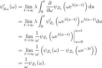
Taking the limit yields

We recognize this as the characteristic function of a ![]() gamma distributed random variable as previously claimed.
gamma distributed random variable as previously claimed.
Construction via the Stationary Distribution
Without assuming a particular form of the background driving Lévy process ![]() , we start from
, we start from
![]()
as above. Let

be the cumulant generating function of the stationary distribution of ![]() . Then (not being fully rigorous)
. Then (not being fully rigorous)

This relationship between the cumulant generating function of the stationary distribution of ![]() and the cumulant generating function of the background driving Lévy process has been obtained by Barndorff-Nielsen (2001). Now, given that the stationary distribution of
and the cumulant generating function of the background driving Lévy process has been obtained by Barndorff-Nielsen (2001). Now, given that the stationary distribution of ![]() is
is ![]() with
with
![]()
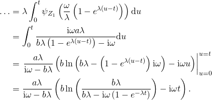
we get

As shown before, this is the cumulant generating function of a compound Poisson process with arrival rate ![]() and i.i.d. exponentially distributed increments with mean
and i.i.d. exponentially distributed increments with mean ![]() .
.
Integrated Time-Change
As shown in my previous post, the general solution for the characteristic function of the total activity process ![]() is given by
is given by
![]()
The integral evaluates to

Putting everything together, we get
![]()
This coincides with the expression given in Chapter 7.2 of Schoutens (2003).
References
Barndorff-Nielsen, Ole E. (2001) “Superposition of Ornstein-Uhlenbeck Type Processes,” Theory of Probability and its Applications, Vol. 45, No. 2, pp. 175-194
Barndorff-Nielsen, Ole E. and Neil Shephard (2001a) “Modelling by Lévy Processes for Financial Econometrics,” in Ole E. Barndorff-Nielsen, Thomas Mikosch and, and Sidney I. Resnick eds. Lévy Processes – Theory and Applications: Birkhauser, pp. 283-318
Cont, Rama and Peter Tankov (2004) Financial Modelling with Jump Processes: Chapman & Hall
Schotens, Wim (2003) Lévy Processes in Finance: John Wiley & Sons
